A Comprehensive Guide on How to Create Drop Down List in Excel

There are many instances when users need more time to enter all the data manually in Excel workbooks. However, if you want to get out of this problem, there are many ways to try. But to create a drop-down list in Excel is the most effective and proven method that is relatively easy to apply. This feature enables users to avoid any data entry hassle.

In addition, a drop-down list is used in spreadsheets to enter the data from already defined cells. The main purpose behind applying a drop-down list is to limit the particular data to the users. So, explore this article till the end and learn different methods to enter the drop-down list.

Part 1. How to Create a Drop-Down List in Excel With and Without Data Validation?

Creating a drop-down list in Excel can greatly enhance data entry and organization. Whether you prefer to use data validation or explore alternative methods, there are multiple ways to achieve this functionality. Here, we will help you learn about the two methods to help you manage tasks and improve efficiency.

With Data Validation

When creating a drop-down list in Excel, the data validation method can provide a reliable and straightforward solution. Follow the steps below to help you carry out the task easily:

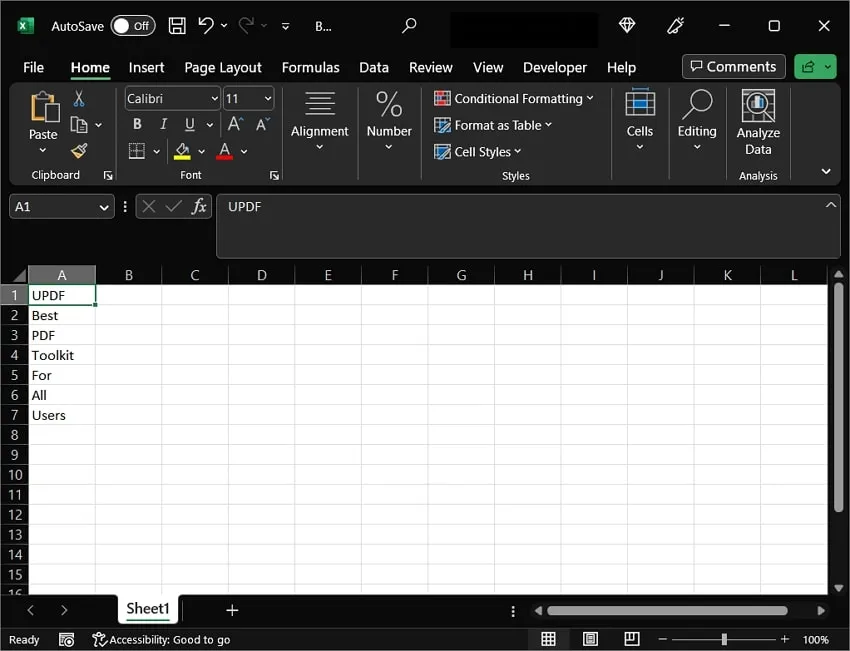
Step 1: Start by locating and accessing the Excel sheet from your computer. Afterward, finalize the cells where you want to add the drop-down list feature.

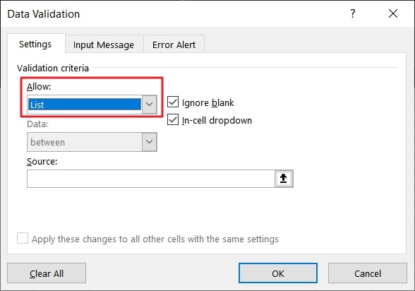
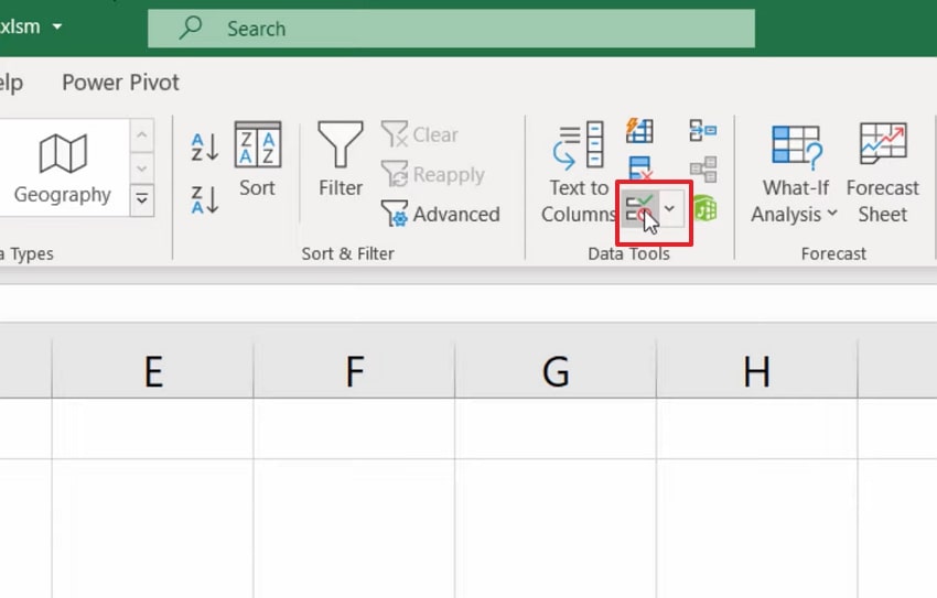
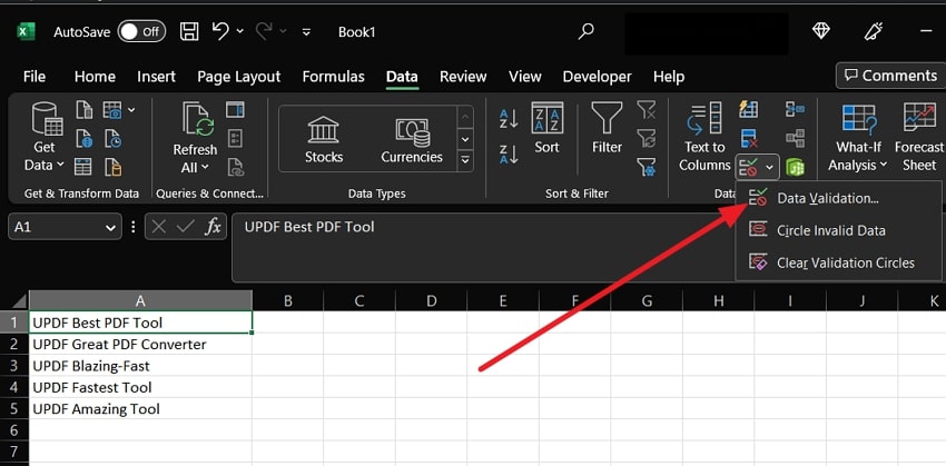
Step 2: Now, head to the “Data” tab, and then select the "Data Validation" option from the "Data Tools" group. This will open a "Data Validation" window. Then, under the "Validation Criteria" section, select the "List" option in the "Allow" box. Following this, ensure that the "In-cell Drop-down" box is enabled.

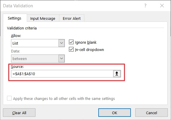
Step 3: Moving on, in the “Source” box, select a range of cells that you want to appear in the drop-down list. Afterward, press the “OK” button to confirm the changes.

Without Data Validation

However, bypassing data validation opens up various new methods if you are looking for an alternative approach to creating a drop-down list in Excel. Head to the steps below to insert a drop-down list without the use of the data validation feature:

Instruction: Move your cursor and select the last cell where the data ends. Now, to apply a drop-down list, press the “Alt” key and downward arrow key on your keyboard.

Part 2. How to Create a Drop-Down List in Excel From Another Sheet?

Managing a drop-down list in Excel from another sheet can be useful for overlooking data entry and ensuring consistency. By linking the drop-down list to a separate sheet, you can easily update and manage the list's options without directly editing the data in the main sheet. Follow the steps below:

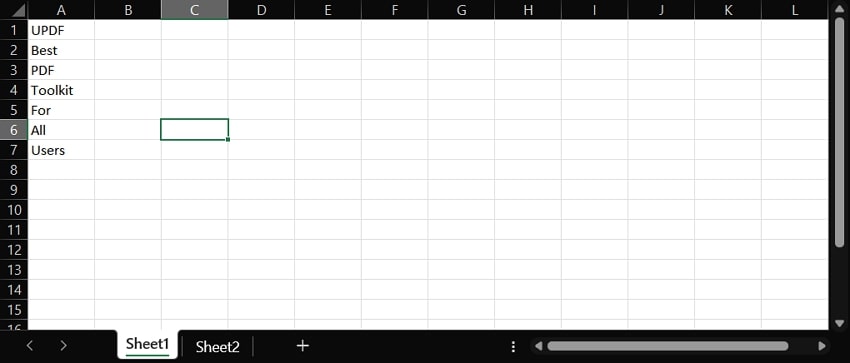
Step 1: Open the Excel workbook and add the data that you want to use to create your drop-down list. Now, select the entire column by clicking on the column header. However, selecting the entire column instead is important so that any new data you add later will be included in the drop-down list.

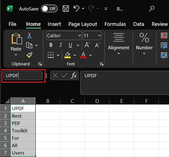
Step 2: In the “Name Box," give the range a name that you will use to reference it later. For example, if you're creating a drop-down list of clothing items, you could name the range "UPDF ."Then, press the Enter key on your keyboard when you are done.

Step 3: Then, go to the sheet and select the cell where you want the drop-down list to appear. Following this, on the ribbon, select the “Data” tab. In the “Data Tools” section, locate and proceed with the “Data Validation” tool.

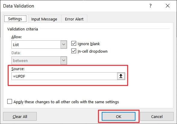
Step 4: When the “Data Validation” dialog box opens up, stay on the “Settings” tab. However, in the “Allow” section, select “List” from the drop-down menu. After that, in the “Source” section, type the equal sign followed by the name of the range you created in Step 2. For example, if you named your range "UPDF," you would type "=UPDF." Finally, click the "OK” button to make the drop-down list.

Part 3. How to Create a Drop-Down List in Excel with Multiple Selections

Enhancing data entry capabilities in Excel is made easier by creating a drop-down list with the ability to select multiple options. This feature allows users to choose multiple items from a predefined list, providing flexibility and efficiency in various tasks such as project management, surveys, and data organization. Explore the below steps:

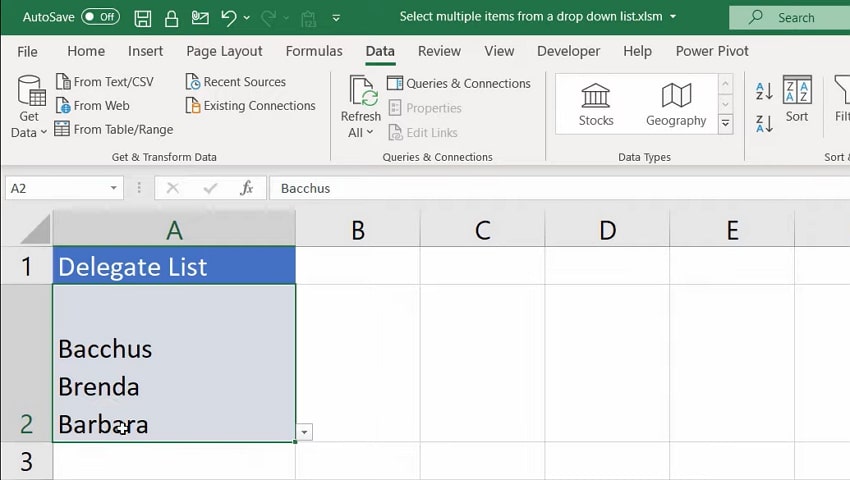
Step 1: Initially, open the desired Excel worksheet. Continue by selecting the cells that you want to include in the list. Now, locate the “Name Box" just to the formula bar's left. This box displays the default cell address created by Excel of the active cell. Following this, click inside the “Name Box” and type a name for your list.

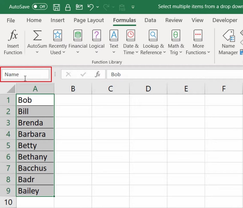
Ensure the name starts with a letter and contains no spaces. After that, press the Enter key on your keyboard to confirm the list's name.

Step 2: Following this, select the cell or cells where you want the drop-down list to appear. Navigate to the “Data” tab on Excel's ribbon at the top of the screen. Next, press the “Data Validation” icon in the “Data Tools” section. The Data Validation dialog box will appear on the spot.

Step 3: Now, in the "Allow" section of the dialog box, select "List" from the drop-down menu. Moving forward, click inside the "Source" box. Here, insert the equal sign and then type the name of your cell range.

Step 4: Finally, click the "OK" button to close the dialogue box. Next, use the "ALT+F11" keyboard shortcut to launch the Visual Basic Editor. Ensure that the Project Explorer is visible. In the Project Explorer window, choose the Excel worksheet that contains your drop-down list.

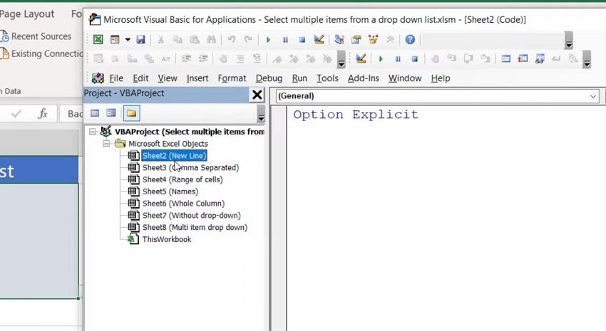
Step 5: After that, copy and paste the following code into the Code window.

Option Explicit

Private Sub Worksheet_Change(ByVal Destination As Range)

Dim DelimiterType As String

Dim rngDropdown As Range

Dim oldValue As String

Dim newValue As String

DelimiterType = ", "

If Destination.Count > 1 Then Exit Sub

On Error Resume Next

Set rngDropdown = Cells.SpecialCells(xlCellTypeAllValidation)

On Error GoTo exitError

If rngDropdown Is Nothing Then GoTo exitError

If Intersect(Destination, rngDropdown) Is Nothing Then

   'do nothing

Else

  Application.EnableEvents = False

  newValue = Destination.Value

  Application. Undo

  oldValue = Destination.Value

  Destination.Value = newValue

    If oldValue = "" Then

      'do nothing

    Else

      If newValue = "" Then

        'do nothing

      Else

        Destination.Value = oldValue & DelimiterType & newValue

        ' add new value with delimiter

      End If

    End If

End If

exitError:

  Application.EnableEvents = True

End Sub

Private Sub Worksheet_SelectionChange(ByVal Target As Range)

End Sub

Step 7: At the end, close the Visual Basic Editor (VBE). You should now be able to select multiple items from your drop-down list.

Part 4. How to Create an Excel Drop Down List with Search Suggestions?

Excel drop-down lists are a powerful tool for data validation, but what if you want to enhance them further by adding search suggestions? With creativity, you can create an Excel drop-down list with search suggestions to improve user experience. Refer to the steps guided below to implement this useful functionality in Excel:

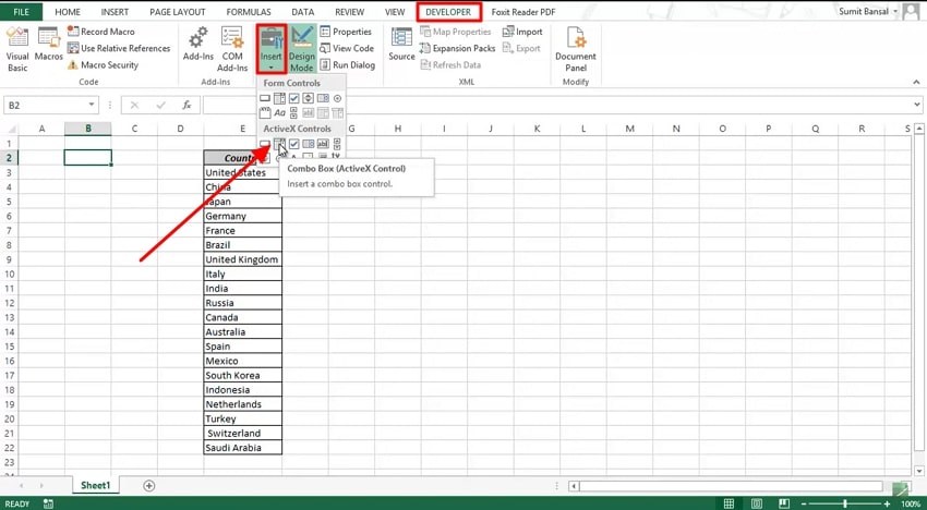
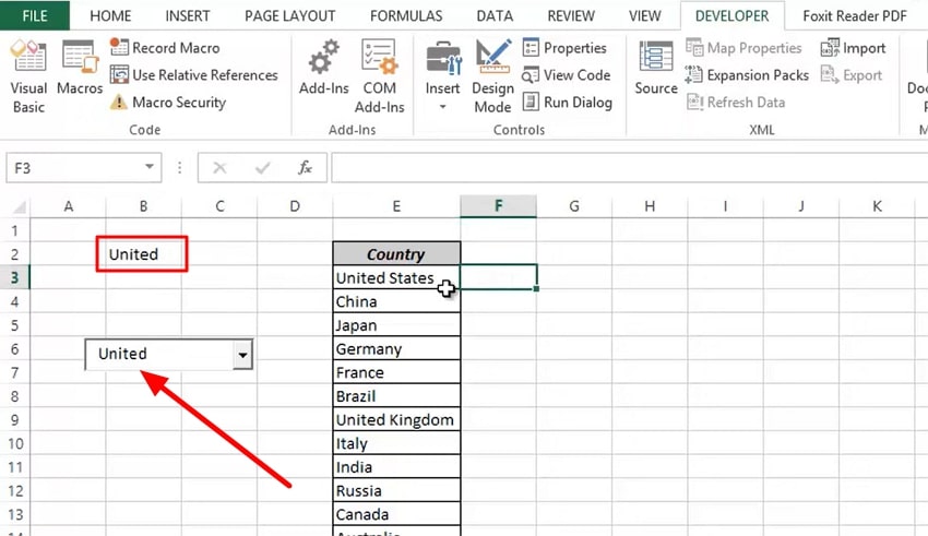
Step 1: At the beginning, go to the “Developer” tab in the Excel ribbon. After that, click on the "Insert" button in the “Controls” group. Then, from the drop-down menu, find the "ActiveX Controls" section and then locate the "Combo Box (ActiveX Control)" icon and select it.

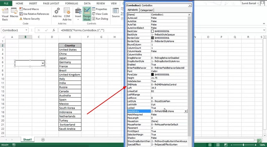
Step 2: Move your cursor to the worksheet area and click anywhere to insert a combo box. Now, right-click on the combo box and select the "Properties" option. In the dialogue box, navigate to the “Alphabetic” category and make the following changes:

• Set "AutoWordSelect" to False.
• Set "LinkedCell" to B2.
• Set "MatchEntry" to 2 - fmMatchEntryNone.

Step 3: Close this dialogue box, return to the Developer tab, and click "Design Mode." This will enable you to enter text in the combo box. Also, since cell B2 is linked to the combo box, any text you enter in the combo box will be reflected in B2 in real time.

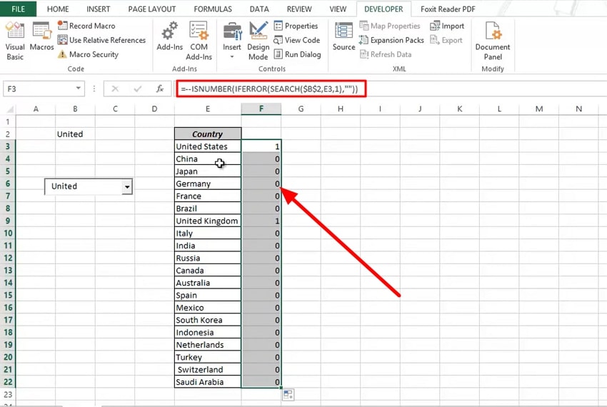
Step 4: Now that the search box is set up, insert the following formula in cell F3 and drag it down for the entire column (F3:F22).

• =--ISNUMBER(IFERROR(SEARCH($B$2,E3,1),""))

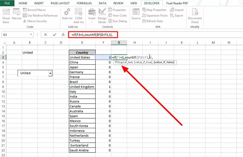
Step 5: Insert the formula in cell G3 and drag it down for the entire column (G3:G22).

• =IF(F3=1,COUNTIF($F$3:F3,1),"")

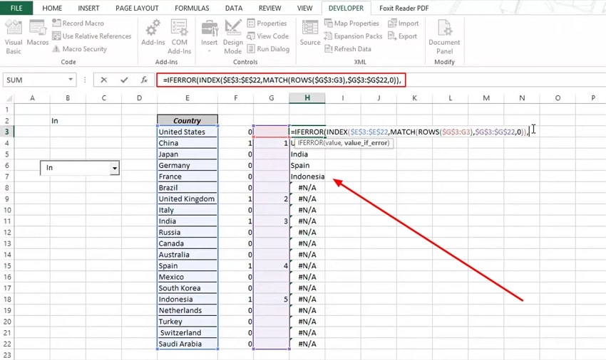
Step 6: Insert the following formula in cell H1 and drag it down for the entire column (H3:H22):

• =IFERROR(INDEX($E$3:$E$22,MATCH(ROWS($G$3:G3),$G$3:$G$22,0)),"")

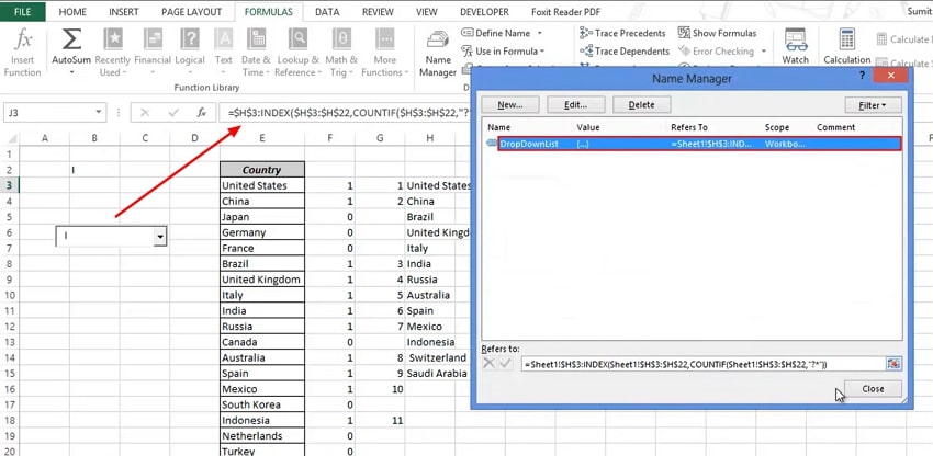
Step 7: Now that the helper columns are set up, we must create a dynamic named range. Go to the “Formulas” tab and click on "Name Manager" in the “Defined Names” group.

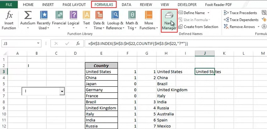
Step 8: In the Name Manager dialogue box, click "New" to open the “New Name” dialogue box. Then, in the Name field, enter "DropDownList ."In the Refers to the field, enter the following formula and close the dialog box.

• =$H$1:INDEX($H$1:$H$20,MAX($G$1:$G$20),1)

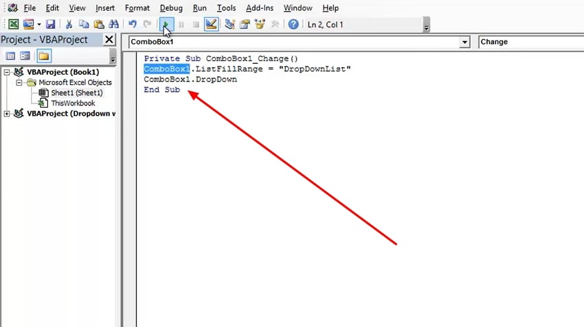
Step 9: Finally, right-click on the worksheet tab and select "View Code." Then, in the VBA window, copy and paste the following code.

Private Sub ComboBox1_Change()

ComboBox1.ListFillRange = "DropDownList"

ComboBox1.DropDown

End Sub

Part 5. How to Create Drop Down List in Excel with Color?

To enhance the visual appeal of your Excel spreadsheets, you can create drop-down lists with color coding. By adding color to your drop-down lists, you can make them more visually distinguishable and easier to navigate. Carefully follow each step to achieve this task:

Step 1: Start by making a list of data and decide on a range where you want to place the drop-down list values. Afterward, click on the "Data" tab, then select "Data Validation," and choose "Data Validation" again from the drop-down menu. In the "Data Validation" dialogue box, click on the "Settings" tab and select "List" from the drop-down menu labeled "Allow."

Step 2: Next, choose the "Source" option, enter the cell range, and click "OK." You should now see the drop-down list below. To add color to the drop-down list, select the cells where the drop-down list is located. Then, go to the "Home" tab and click on "Conditional Formatting," followed by selecting "New Rule."

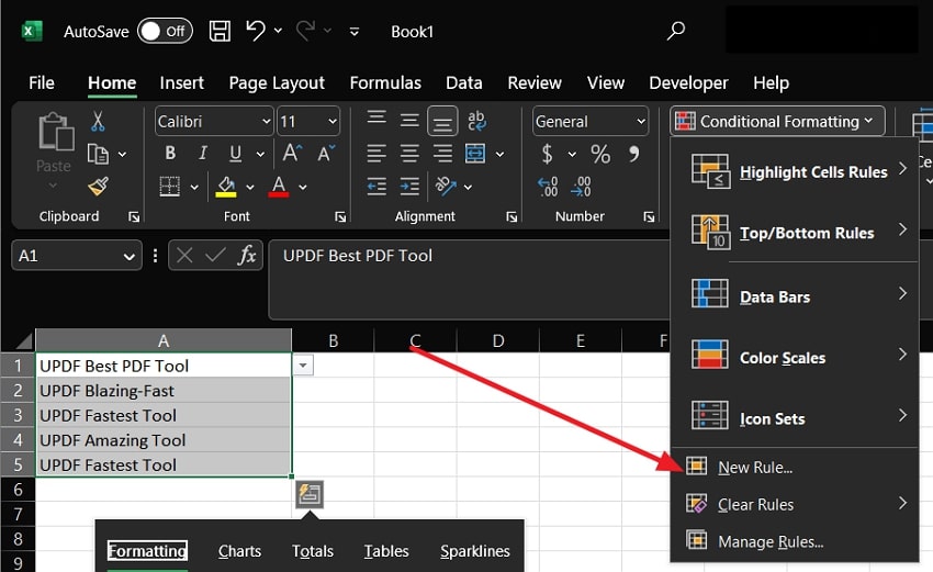
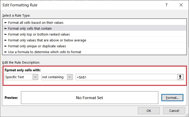
Step 3: In the "New Formatting Rule" dialog box that appears, click on the "Format only cells that contain" option under the "Select a Rule Type" section. Under the "Format only cells with" section, choose "Specific Text" from the first drop-down list and desired option from the second drop-down list. After confirming all the rule settings, click on the "Format" button.

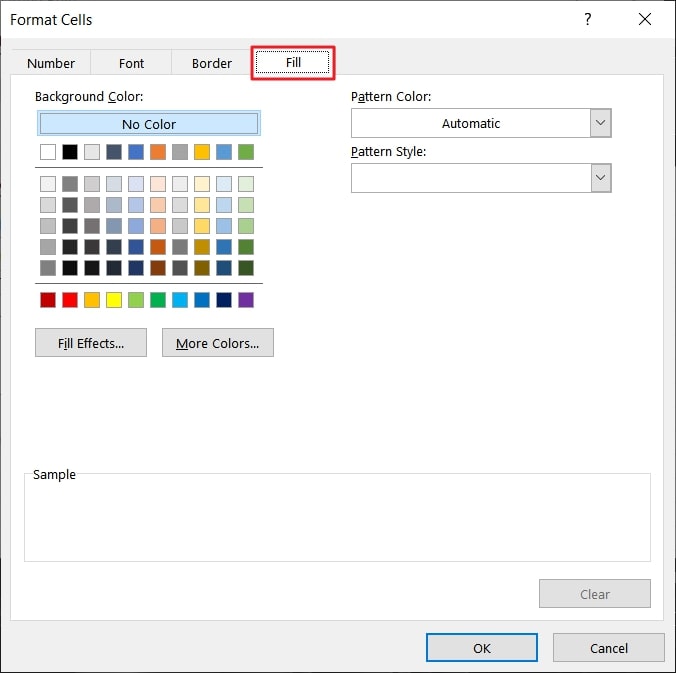
Step 4: In the "New Formatting Rule" dialog box, click the "Fill" tab and choose the desired color. Next, click "OK" to close the dialog box. After that, confirm the new rule by pressing the "OK" button, and it will fill the cells according to the rule you have set.

Part 6. How to Create a Drop-Down List in Excel with If Statement?

As you know that Excel provides a useful feature called data validation, through which you can create drop-down lists for streamlined data entry. By incorporating the IF statement, you can take this functionality further by modifying the available options based on specific conditions. Here, learn how to create a drop-down list with an IF statement in Excel:

Step 1: First, click on the desired cell where you want to add the drop-down list. Then, in the Ribbon at the top of the screen, go to the “Data” tab. From the “Data Tools” section, choose “Data Validation.”

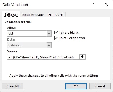
Step 2: Then, in the “Data Validation” dialog box that appears, select the "List" option from the "Allow" drop-down box. In the "Source" field, type or enter the formula specifying available range names.

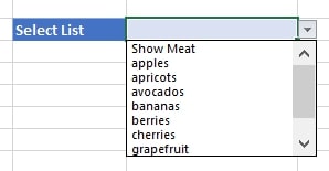
• =IF(C2="Show Fruit", ShowMeat, ShowFruit)

Step 3: Now, click the “OK” button to confirm the data validation settings. Now, you will notice a small drop-down arrow next to your selected cell. Next, click on the drop-down arrow to open the list of available fruits.

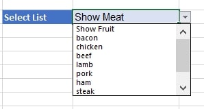
Step 4: However, if you want to switch to the meat list, click "Show Meat" or an appropriate option. After selecting the "Show Meat" option, click on the drop-down arrow again. Here, you will observe that the list has changed to show the meat options, while the top value in the drop-down box will have changed to "Show Fruit" or any relevant indication.

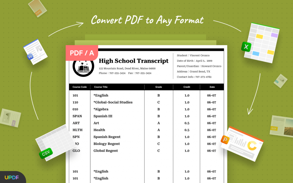
Part 7. How to Extract Data From PDF to Excel When Creating a Drop-Down List in Excel

UPDF is a powerful PDF editor tool that offers a convenient solution for extracting data from PDF files. If the files contain drop-down lists, this tool can convert them into Excel format. With UPDF, you can easily retrieve information from PDF documents and transfer it to an Excel spreadsheet. Moreover, this tool ensures accuracy and efficiency, so your data isn't damaged.

This tool enables swift data extraction and allows you to make necessary edits to the content. Luckily, giving you full control over the converted file. Whether you need to extract data from forms or any other PDF document with drop-down lists, UPDF simplifies the process with enhanced productivity.

Steps to Help You Convert PDFs into Excel Spreadsheets

If you want to convert your PDF files, follow the detailed steps below so that you do not face any inconvenience:

Step 1: Open the PDF File Containing Required Data

Locate the UPDF tool on your device and double-click to open it. Now, tap the “Open File” option to find and import the desired file that contains the drop-down list.

Step 2: Select the File Format to Convert PDF To

After the file is open, move the cursor to the right sidebar and select the "Export PDF" option. From the available supported formats, choose "Excel (.xlsx)" format.

Step 3: Customize the Conversion Settings

Here, choose the "Output Format" as Excel, select the "Page Range," and tap the "Export" button. On the new window, select the destination folder and save your file in the Excel format.

Final Words

Creating a drop-down list in Excel is a straightforward process that can greatly enhance your data entry and analysis capabilities. By following the steps outlined in our detailed article, you can easily create drop-down lists and improve the efficiency of your spreadsheets. Before setting it up, remember to carefully consider the list items and their relevance to your data.

Additionally, if you have existing PDF files that contain drop-down lists and need to convert them into Excel format, we recommend using the UPDF tool. This tool offers a convenient and user-friendly solution to convert PDF files. Using this tool, users can avoid the need for complex file conversion methods.