How to Compare Two Excel Sheets? Easy Ways

Microsoft Excel is one of the best spreadsheet tools, and since it allows you to have multiple sheets in one document, things can get even better. However, sometimes you need to compare sheets for different or duplicate values in data, and depending on the data size, that can be very time taking if you don’t know the right process. Learn how to compare two Excel sheets smartly to save time and effort.

Let's elaborate on the top 5 easy ways for comparing 2 different Excel sheets to find any data that is different or duplicated between them. The best part about using these methods is that they save you time.

Part 1. How to Compare Two Excel Sheets for Differences and Duplicates With "Arrange All"?

The first method we will share here is the Arrange All function of Microsoft Excel. This method is considerably easier than other methods, and the setup takes less time and steps. So, here are all the steps to follow for using Arrange All method:

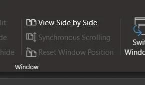
• Open the file and Excel sheets you want to compare and open the View tab. So, now click the "side-by-side" button. Remember that this button is only available if multiple Excel spreadsheets are open.

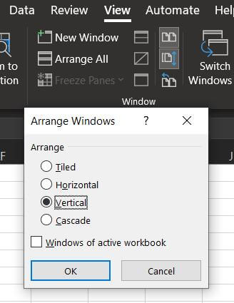
• Excel spreadsheets will, by default, appear in a horizontal orientation. So, you need to click the Arrange All button and select Vertical.

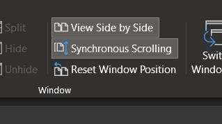
• To make comparing easier, the last thing you need to do is enable synchronous scrolling in the view section. With this option enabled, both sheets will scroll together.

This method is effective whether you compare two sheets in two Excel documents or within the same document. Additionally, use this method when working with a small dataset since human error is possible. However, this method will still increase your efficiency by saving time.

Part 2. How to Compare Two Excel Sheets for Duplicates or Differences With "New Window"?

Another method to compare data in Excel sheets is the New Window method. It is specifically beneficial when you have one workbook and different spreadsheets in them. Alternatively, you can select different Excel workbooks and compare them to check for differences or duplicates.

It is only possible due to the New Window feature from Excel, and the method is simple and similar to the previous one. Let's take the example of one workbook with 2 spreadsheets in it that you will compare with the following steps:

• After opening the workbook that contains spreadsheets, you need to open the View tab, and inside it, you will click on the New Window button. It will open another window for the same Excel worksheet.

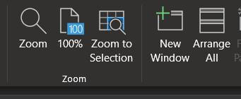
• If the orientation of these windows is horizontal, but you want to compare data in columns, you can click on the Arrange All button to select the vertical orientation.

• Moreover, if you compare spreadsheets with long data columns, enable the synchronous scrolling option in the view tab. It makes both spreadsheets scroll together, ensuring the rows stay the same when you compare.

This method is better for small datasets since you will manually compare the data. There is a high chance of facing human error while comparing the data. Additionally, it works exceptionally well when you have one workbook with two spreadsheets in it.

Part 3. How to Compare Two Excel Sheets and Highlight Differences?

One thing common about the previous two methods is that you manually compare the data. That is only possible if you have a small number of rows in each column. If you have longer columns, you may face several errors in that method, making it important to choose a smart way. So, instead of doing things manually, use smart tools from Excel to compare the differences.

The best part about it is that it highlights the differences. However, having the spreadsheets in one workbook is essential as you can’t compare spreadsheets between 2 workbooks with this method. If you have spreadsheets in multiple workbooks, you can copy them into one.

To better understand the steps, we will take the example of 2 datasets, with one having new student scores and the other having old scores. It uses the Conditional Formatting feature, and here are the steps to implement this method:

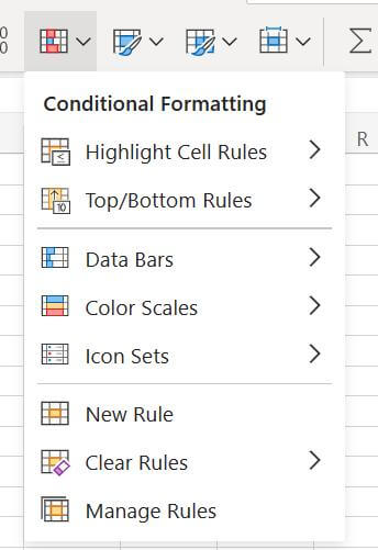
• Select the data in the "New" sheet and open the home tab, then click on conditional formatting, then new rules.

• In the rules section, you must select the last option that uses a formula for determining cells to format and enter the formula “=B2<>Old!B2". Update the formula according to your column and spreadsheet name.

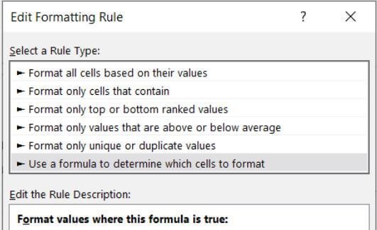
After you enter the formula, press the format button. Lastly, pick a color from the Fill tab in the popup window and click OK. Now you will see the different values will instantly be highlighted.

Part 4. How to Compare Two Excel Sheets and Highlight Differences Online?

Use an even smarter solution if the previous method is hard to work with. That solution involves using an online tool known as Google Sheets. It is a tool that allows you to import xlsx files on it. Since both follow the spreadsheet interface, it similarly displays your Excel workbook.

However, it works with the same conditional formatting technique, but the experience is different. The comparison here is done in one phase, while the highlighting is done in another. Say that you have uploaded your Excel workbook with 2 spreadsheets to Google Sheets and opened it; now you can follow the steps below to find differences:

• Click any empty cell and type an equal sign. Then you want to click on the cell from the first spreadsheet you want to compare. Again, type the equal sign, go to the second spreadsheet in this document, and click on the first-row data cell. Hit enter, and you will see true/false appear.

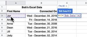
• Now copy and fill that formula by dragging down the right corner of that cell. You will see true/false appear in every cell. A true represents equal values in the selected cells, while a false indicates different values.

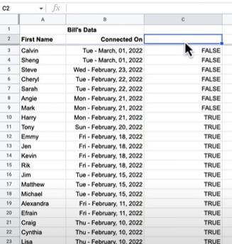
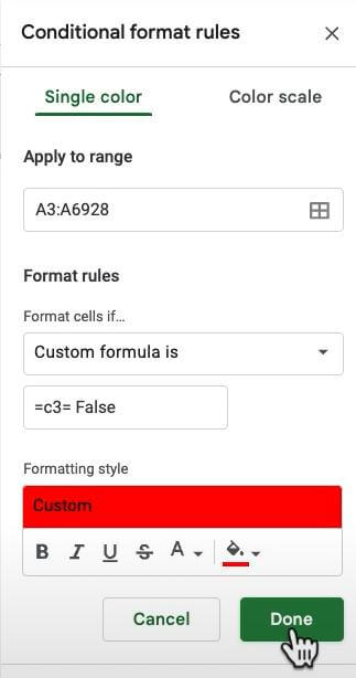
• Select the column whose data you are comparing. From the top menu, click on format and select conditional formatting. In the "format cells if" option, select the conditional formula. In the formula bar, you will enter "=C3=F".  C3 is the column that represents True/False, and if you use some other column for that, replace C with that and 3 with the first entry of that column. Lastly, you need to pick a color and click Done.

Now you will see that all the different values are highlighted instantly.

Part 5. How to Compare Two Sheets in Excel for Matches and Highlight Them?

Previously we have discussed ways to find the different data to highlight it. Let's share how you can find the matching data or duplicate between sheets and highlight it. The process is very simple since it also uses conditional formatting. The only thing that we will change here is the formula. All the steps and processes will also be the same.

However, for this method to work, having both sheets in one Excel workbook is essential since conditional formatting does not work if the data is present in 2 workbooks. A solution to that is copying the data into a new sheet in the workbook that you are using. We will take the same example of new and old sheets containing student scores. So, find matching data and highlight them using the following steps:

• Select the data in the "New" sheet by dragging the mouse over it. Click the home tab, conditional formatting, and then on new rules.

• In this screen, select the option to use the formula for determining cell formatting. Type the formula “=B2=Old!B2". Update the formula according to your column and spreadsheet name.

As you finish the process, you will see the highlighted matching values.

Part 6. Bonus Tip: The Best PDF to Excel Converter

Say that someone sent you a spreadsheet to compare some data, but that spreadsheet is saved in PDF format. You need that spreadsheet in xlsx format to use the best-comparing features possible with UPDF. It is your best PDF-to-Excel converter since it provides an instant experience.

The best part is that you can edit that spreadsheet as a PDF, share it, divide it into different files, and use many other features like:

• Instant PDF conversion: Convert PDF to any formats.
• Password-protecting PDF spreadsheets, etc.
• Cloud storage with UPDF Cloud
• Add Comments to PDF
• Organize PDFs via replacing, deleting, reordering,, and more.
• OCR PDF

With all these benefits and many others, UPDF is your best choice for converting PDF to Excel.

In The End

You will waste a lot of time and effort if you don’t know how to compare two Excel sheets the smart way and do that manually. Hopefully, you have learned the most effective ways above and selected the one you think would work the best for you.

Sometimes you receive Excel data in the form of a PDF file. That PDF file contains all the spreadsheets, and comparing becomes significantly difficult. Not anymore, use UPDF for the conversion. It instantly converts your files while maintaining data integrity.